Carbon-Dioxide System Relief Sizing

WILLIAM GREULICH, KENSINGTON CONSULTING

CILLERS KRUGER, KORF TECHNOLOGY, LTD

ABSTRACT

Generally, safety standards for refrigeration systems require the placement of at least one overpressureprotection device on all carbon-dioxide (R-744) systems as well as on vessels manufactured in accordance with the American Society of Mechanical Engineers Boiler and Pressure Vessel Code, Section VIII Division I, or the regional equivalent1,2. The standards contain equations for determining the required discharge capacity to relieve pressure caused by external heating for common pressurized system components in the form of a constant multiplied by an area, either projected or actual, specific to the equipment type. The constant in the equations, ƒ, is based on the continuous and constant external radiative heating of two phases in equilibrium at the relieving pressure, allowing for boiling and assuming ideal-gas behavior to convert the boiling mass flow into standard-air flow. In practice, many carbon-dioxide refrigeration systems discharge under non-ideal conditions. Therefore, the underlying assumptions of the current standards do not apply to the real-world conditions that are anticipated for many, if not all, carbon-dioxide refrigeration systems. This study presents an overview with examples of a rigorous twostep isobaric–isentropic calculation method, commonly known as the homogenous direct integration method, to determine the overpressure-protection device maximum flow area for any carbon-dioxide relief condition that may be expected in refrigeration systems.

Summary

The sizing of overpressure-protection devices, which are required for discharging in various fluid states due to the pressure caused by external heating, has been welldescribed in the literature.³ The published work contains background information concerning the inapplicability of relief sizing equations that are derived from idealgas assumptions because the fluid is not expected to be ideal, e.g., in the supercritical region, and describes a widely applicable, rigorous, isobaric–isentropic calculation method. The homogeneous direct integration (HDI) method can be applied to any homogenous equilibrium fluid that reduces pressure along an assumed isentropic path. The method identifies the maximum mass flux under the choked flow condition. Based on the expected mass flow rate, the maximum required relief device flow area can be calculated.

Herein, the HDI method is applied to closed carbon-dioxide systems discharging in the range of 5-20 MPa (700-3,000 psi).

The key to implementing the method is the availability of carbon-dioxide state properties, which can be obtained from the NIST Reference Fluid Thermodynamic and Transport Properties Database (REFPROP). ⁴

The results are presented in a form that can be readily used by industry practitioners worldwide and potentially included in future editions of safety standards.

System Under Consideration

The case considered here is a closed (blocked-in) vessel containing carbon dioxide subjected to an external heating rate of Q = 1.0 kJ/s. This Q value is used for simplicity and subsequent application in any desired basis relationship to determine external heating loads. Calculations are performed at the discharge pressures, ignoring any potential inaccuracy in the device caused by dynamic effects that may occur during device operation, such as potential relief valve chatter or pressure accumulation in the system. Heat transfer effects, such as vessel shell conduction or inefficiency in internal vessel-surface heat transfer, are also neglected. The carbon dioxide is assumed to remain in thermodynamic equilibrium, ignoring any boiling or condensation delay effects. Liquid and vapor phases have the same velocity, and we only consider the no-slip condition. Lastly, no flow area coefficients are included.

Regardless of the initial process conditions, the closed vessel contents are externally heated at the fixed vessel volume, i.e., isochorically, until reaching the relieving pressure.Step 1, the first calculation step of the method, occurs while constant heating is continued at the constant relieving pressure, i.e., isobarically. Step 2, the second calculation step, occurs while the fluid depressurizes at constant entropy, i.e., isentropically. The solution method is iterative, with the results of step 1 feeding into step 2, which returns for refinements of step 1.

Step 1: Isobaric Process at Relieving Pressure

After reaching the relieving pressure, the carbon dioxide continues heating, thus creating the relieving mass flow. This flow may be caused by boiling, if two phases exist, or from single-phase volumetric expansion from the constant vessel volume.

The boiling mass flow rate, which forms the basis of current safety standards, is given by the ratio of heating to the latent heat of vaporization for the relieving condition. For this expression, we can add the conventional correction term for volume change of the two phases during boiling in the fixed volume vessel, ⁵  which is neglected by many safety standards.⁶

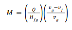
M = Mass relief rate (kg/s)

Q = Heating (kJ/s)

Hfg = Latent heat of vaporization (kJ/kg)

v = Specific volume (m3/kg)

f = Liquid

g = Vapor

Volumetric expansion mass flow, applicable to any single-phase system, is given by⁵

β = Coefficient of volumetric expansion at constant pressure (K-1)
C p = Specific heat at constant pressure (kJ/kg K)

As a preliminary first step for a two-phase system, it is important to determine whether boiling is the dominant mass flow process. Table 1 shows the two values with 1-kJ/s heating for the range of potential two-phase relieving pressures.

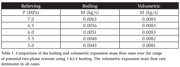
The results of the comparison are convenient because they suggest that volumetric expansion is the dominant source of mass flow, which determines the largest required flow area of the pressure-relief device. As a practical matter, this condition is considered for a vessel that has either exhausted the available liquid by boiling or does not produce a second phase at the relieving pressure.

With this result, all subsequent mass flow rates will be determined using the volumetric expansion approach.

The objective is to determine the maximum allowable flow area of the pressure-relief device, i.e., the flow area at the narrowest cross section when the pressure-relief device is fully open. It is now convenient to introduce the relationship between mass flow rate and flow area, i.e., the expression we intend to maximize,7 which can be expressed as

A = Flow area (m2)
G = Mass flux (kg/s-m2)

In addition to the equations for flow area and mass flow, based on volumetric expansion, applicable to all systems under consideration, it is necessary to define the expression for the required mass flux.

Step 2: Isentropic Process of Depressurization

The fundamental equation for mass flux along a frictionless path follows Euler’s equations of motion. For one-dimensional flow, the expression can be rendered in multiple forms, two of which are examined here. The first is ⁷

u = Velocity (m/s)

This yields

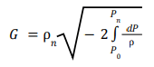
ρn = Density (kg/m3 )

Pn = Outlet pressure (Pa)

P0 = Inlet pressure (Pa)

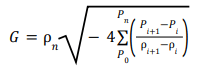
Unfortunately, the integral in the mass flux equation does not have a closed-form solution for non-ideal systems; therefore, a numerical integration technique must be applied. The mass flux equation can be numerically integrated by applying a finite difference method as

However, for adiabatic flow, a second form of the one-dimensional flow equation is also useful, which can be expressed as

This expression can also be integrated as

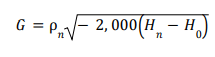
Hn = Outlet enthalpy (kJ/kg)

H0= Inlet enthalpy (kJ/kg)

This second form is more general than the first because it is not restricted to only the isentropic case. However, though it is easier to implement computationally, the sensitivity to small variations in enthalpy means that the accuracy of the enthalpy values are more critical.

We evaluated the range of pressures using both forms and found no significant differences between the results. Therefore, moving forward, only the calculations and results based on this second adiabatic form are presented.

Calculations

The calculations were performed using Excel with a VBA script. The Excel REFPROP wrapper makes this platform particularly convenient.

Tables 2 and 3 provide representative outputs of the calculation method for the relieving pressure of 12 MPa.

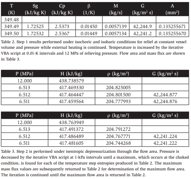
Table 2 shows the final position of the iteration for the relieving pressure of 12 MPa. The carbon-dioxide single-phase entropy at 12 MPa and 349.49 K is 1.72525 kJ/kg K. This entropy value informed the upper panel of Table 3, and the entropy value of 1.72532 informed the lower panel of Table 3. Table 3 also shows the final position of the iteration for the case at 12 MPa. At the flow area pressure of 6.512 MPa, the top panel produced the maximum mass flux value of 42244.877 kg/m2 s, which was returned to Table 2. The bottom panel returned a value of 42241.224 kg/m2 s at 6.512 MPa, which was also returned to Table 2.

Returning to Table 2, the maximum mass flux values are used in conjunction with the calculated mass flow rate to calculate the associated flow areas. At the temperature of 349.49 K, flow area pressure of 6.512 MPa, relieving pressure of 12 MPa, and entropy of 1.72525 kJ/kg K, the maximum flow area of 0.135255671 m2 was obtained.

Notably, all relationships are smooth and continuous, so maxima are easily identified, e.g., the decrease in Table 2 of the area in the final row or the decrease in mass flux in the final row for both Table 3 panels.

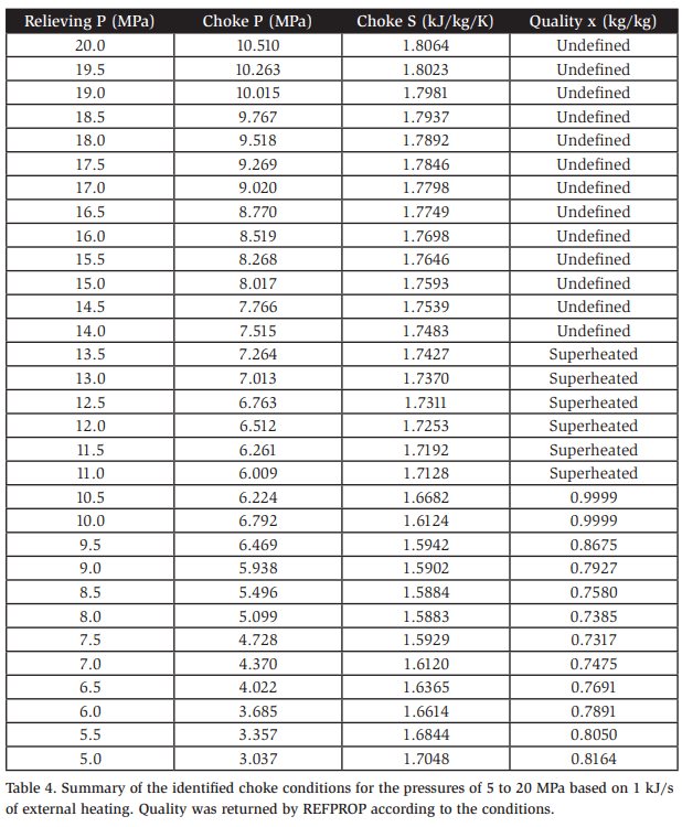
As a practical matter, in all cases, the maximum mass flux, which represents the choked flow condition, was found to be roughly 50% of the inlet pressure, as expected. This is important because this pressure should always be evaluated against any allowable back pressure constraints. Furthermore, it should be confirmed that the choke condition occurs at a pressure above the expected back pressure; if not, then choking will not occur. Table 4 shows the choke conditions calculated for the examined pressure range.

Finally, no formal error analysis was undertaken. However, the final results represent heating temperature steps of 0.01 K and depressurization steps of 1 kPa. A casual examination of the sensitivity from varying these factors indicates that the final temperature and pressure resolution is likely more than adequate. Additionally, as indicated earlier, results from the two forms of the mass flux equation produced nearly identical results. Deviations were much less than 1% under the lowest pressure conditions.

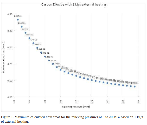
Results

Figure 1 summarizes the maximum flow areas for the range of relieving pressures.

Application

The study was performed on a linearly scalable unit external heating basis of 1.0 kJ/s, making the results generalizable for any desired method of determining external heating.

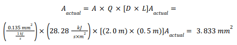
Example 1: Consider a carbon-dioxide refrigeration vessel that is 2 m long and 0.5 m in diameter, relieving at 12 MPa. Based on the heating basis equation contained within the IIAR CO2 Standard for Q = 28.39 kJ/s-m2 applied over the projected area (length x diameter)6 and the maximum flow area of 0.135 mm2 , which is shown in Figure 2 for relieving at 12 MPa, the required actual flow area is

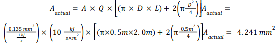
Example 2: Consider the same system but now refer to the European Standard – 378-22 , which requires that Q = 10 kJ/s-m2 is applied over the vessel’s total surface area. Then, the required actual flow area is

Areas are also readily converted to standard-air flow rates, which is common for specifying devices in refrigeration services. 

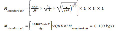
Example 3: Consider the system in the first example. To assist in specifying a relief valve, it is necessary to determine the required capacity for the mass flow rate of air at T = 293.15 K. We can use Fliegner’s formula⁸ for an ideal gas and assume a perfect nozzle, gas constant of R = 287.04 J/kg/K, and specific heat ratio for air of ϒ = 1.4. In addition, we must scale the result by applying the external heating Q = 28.39 kJ/s-m2 over the projected area, i.e., length (m) x diameter (m), which can be expressed as

Conclusion

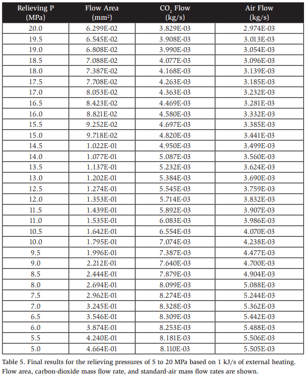
Table 5 shows the maximum flow area, mass flow rate of carbon dioxide, and mass flow rate of standard air evaluated on a unit external heating basis of 1 kJ/s for each relieving pressure. These values can help determine the discharge capacity in accordance with any of the safety standards, provided that their specific requirements are also considered.

To complete a required discharge capacity determination, depending on the chosen safety standard, the appropriate relieving pressure should be chosen based on the allowable pressure accumulation, typically 10% or 21% above the set pressure for most safety standards.

Then, the applicable safety standard format, mass flow of CO2, mass flow of air, or flow area should be adjusted as shown in the examples for determining the equipment size and method of calculating the external heat load.

Finally, any other adjustments, such as the inclusion of discharge or capacity coefficients, should be included as required by the applicable safety standard or indicated by the device manufacturer.

With these simple arithmetic adjustments, the results are obtained in a form that is useful for industry practitioners worldwide and can be potentially included in future editions of any of the global refrigeration safety standards.

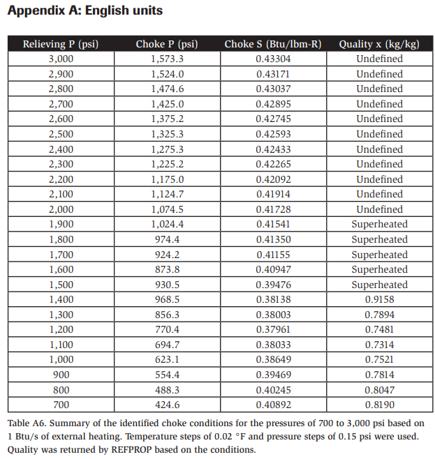
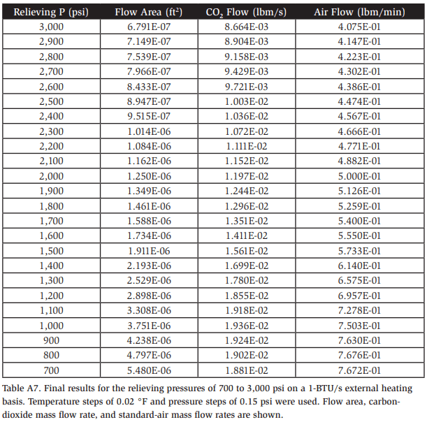
Example A1: Consider a carbon-dioxide refrigeration vessel that is 2 ft long and 0.5 ft in diameter, relieving at 1,700 psi. To assist in specifying a relief valve, we must determine the required capacity in the mass flow rate of standard air. Based on the heating basis equation contained within the IIAR CO2 Standard for Q = 150 Btu/minft2 applied over the projected area (length x diameter)6 and the standard-air flow rate of 0.54 lbm/min shown in Table A7 for 1,700 psi, which was calculated based on 1 Btu/s, the required capacity is

Citations

1.  “Safety Standard for Closed-Circuit Carbon Dioxide Refrigeration Systems.” ANSI/ IIAR CO2, International Institute of Ammonia Refrigeration, Alexandria, VA, 2021.
2.  “Refrigerating Systems and Heat Pumps – Safety and Environmental Requirements – Part 2: Design, Construction, Testing, Marking and Documentation.” CENEN-378-2, European Committee for Standardization (CEN), Brussels, Belgium, 2016.
3. Darby R. “Size Safety Relief Valves for any Conditions.” Chemical Engineering, September 2005.
4. Lemmon E, Huber M, McLinden M. “NIST Standard Reference Database 23: Reference Fluid Thermodynamic and Transport Properties-REFPROP, Version 10.0.” National Institute of Standards and Technology, 2018.
5. “Guidelines for Pressure Relief and Effluent Handling Systems.” American Institute of Chemical Engineers, NY, NY, 1998.
6. Fenton D, Richards W. “User’s Manual for ANSI/ASHRAE Standard 15-2001, Safety Standard for Refrigeration Systems.” American Society of Heating, Refrigerating and Air-Conditioning Engineers, Atlanta, GA, 2003.
7. Darby R, Chhabra R. “Chemical Engineering Fluid Mechanics, 3rd edition.” CRC Press, New York, NY, 2017.
8. Shapiro A. “Compressible Fluid Flow.” The Ronald Press Company, New York, NY, 1953.