Measurement Device Platform Designed for the Performance Assessment of Low-Temperature Blast Freezing Systems

Author: Eric Alar, PhD Candidate at the University of Wisconsin-Madison

Abstract

Air blast freezing systems are among the most widely used technologies for rapidly freezing both packaged and unpackaged foodstuffs. In many food processing facilities, freezing is a bottleneck in the continuous flow production, and thus techniques to assess and improve their thermal performance are of significant interest. Furthermore, there is interest in improving energy performance because blast freezing is among the most energy-intensive processes in packaging plants.

This paper discusses the development and application of an instrumented fixture that can be used to evaluate the thermal performance of dynamic air blast freezers. The device is capable of collecting detailed heat transfer characteristics and air temperatures in situ while being directly conveyed through the freezer, side-by-side with the product. Details of the device are discussed along with the comparative thermal performance of five air blast spiral freezing systems.

Introduction

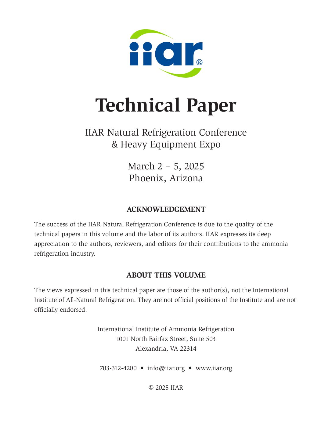
The food and beverage sector constitutes approximately one-third of the global energy consumption and one-fifth of all greenhouse gas emissions (FAO 2011). Approximately 40% of this energy usage is related to processing and distribution, with food retail and preparation compromising another 35%. Notably, “Freezing Equipment” represents the largest investment in the food production line. Lowering the refrigeration temperature in production facilities by 10°F (−12°C) can increase the utility bill by 15% (ASHRAE 2018), underscoring the impact of the freezing system. The number of food processing and distribution facilities is considerably smaller than the number of retail, preparation, and cooking operations. Moreover, these processing centers require high energy, emphasizing the need to improve energy efficiency in food processing and distribution facilities. As a result, the overall energy consumption of this important sector can be effectively reduced. The dominant form of production freezing is air blast freezing (ASHRAE 2018). This paper focuses on the spiral version, a dynamic freezer system that can be directly integrated into the food production pathway. A spiral blast freezer is illustrated in Figure 1.

Air blast freezing systems present interesting and unique challenges from a design standpoint. Fundamentally, the rate of heat removal from food products in a blast freezer is primarily a function of the surface heat transfer coefficient and air temperature. Modern spiral freezers utilize multiple fans to generate high-velocity airflow across products being conveyed through the freezer to increase the product’s air-side heat transfer coefficient; thereby, increasing the rate of heat removal. However, increasing the air velocity requires more electrical power to drive the fans (a cubic relationship), and 100% of the energy used to drive the fans becomes a parasitic thermal load within the freezing system. Lowering the air temperature within the spiral conveyor increases the rate of freezing, but lower air temperatures substantially increase the energy consumption of the refrigeration system that serves the freezing system. Lower air temperatures also require operating costs and/or capital costs of the refrigeration system.

As part of this project, five spiral freezers undergo comparative field evaluation using a measuring device specifically designed to monitor this equipment. Typically, the heat transfer coefficient within a spiral freezer, linking the hot incoming product to the refrigerated air supply, is estimated using values from the ASHRAE Refrigeration Handbook (ASHRAE, 2022). These tables provide heat transfer coefficients for various food products exposed to air velocities below 5 m/s. However, the data in these tables are generalized and often tailored to specific products, with wide variability between examples. This highlights the need for more precise knowledge of both the cooling process and the specific product being processed to accurately predict freezer performance. Although the air velocity in production-scale blast freezers can fluctuate significantly, the prevailing method for modeling the freezing process assumes a constant heat transfer coefficient, as demonstrated by Reynoso and Calvelo (1985) and Mannapperuma et al. (1993).

Accurately measuring and predicting surface heat transfer coefficients for food products has traditionally posed significant challenges, as noted by Amarante et al. (2005) and Lovatt et al. (1993). These studies demonstrated that the heat transfer process during food freezing is inherently complex, making precise measurements difficult. In Amarante’s research, rectangular film heat flux sensors were applied to irregular, curved organic food items (e.g., tomatoes) to estimate heat transfer coefficients. However, the sensor data were calibrated against a Fourier heat transfer model using correction factors, effectively aligning the measurements with the model’s assumptions (Amarante et al., 2005). Thus, the measured heat transfer coefficient closely matched the model’s predictions, suggesting that the measurements were constrained by the model rather than reflecting uncorrected sensor data.

Carson et al. (2006) used similar heat flux sensors on flat plaster surfaces within an oven, comparing the observed heat transfer coefficients with those derived from a model incorporating transient temperature data, a mass-loss rate model, and a psychrometric approach. The heat flux sensors produced heat transfer coefficients that were approximately twice as high as those obtained through the other methods, which was attributed to the influence of radiation effects. Despite this discrepancy, the researchers emphasized that heat flux sensors were likely the most practical tool for obtaining real-time heat transfer coefficient data. The study specifically focused on low air velocities, ranging from 0.1 to 0.7 m/s, within a heating oven environment, rather than a cooling freezer. Sensors were mounted on a lowconductivity plaster medium, where the temperature difference between the plaster surface and the oven air never reached a steady state owing to the absence of a constant temperature or heat flux sink. These findings highlighted both the versatility and potential of heat flux sensors for accurately measuring heat transfer coefficients.

The present paper addresses several challenges encountered in previous studies deploying heat flux sensors to measure heat transfer coefficients in situ, which lacked clear and consistent methods for interpreting signals from heat flux sensors. We propose a simple and effective approach for capturing these measurements, eliminating the need for complex third-party data acquisition systems with uncertain functionality or bulky fixed multimeter devices. Attaching heat flux sensors directly to food surfaces presents additional difficulties because the low structural stability and changes in surface characteristics during processing complicate the heat flux measurement.

This study focuses on measuring the heat transfer coefficient in operating spiral blast freezers by attaching heat flux sensors to an aluminum substrate that exhibits more isothermal behavior. Real-time radiation effects are accounted for using an emissivity estimation method. To demonstrate a practical application, we monitor a surrogate food product conveyed through an operational spiral freezer. The heat transfer coefficient measurements are then used to define the thermal boundary condition in an existing 1D thermal model, and the host freezers are compared, as described in the Results section.

Apparatus, instrumentation, and sensors

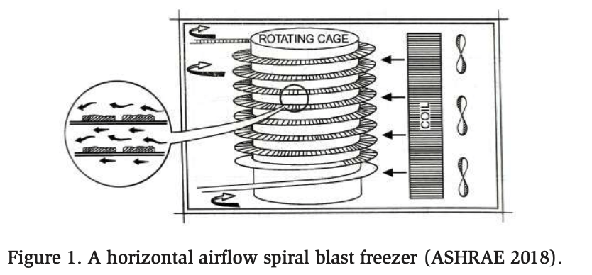
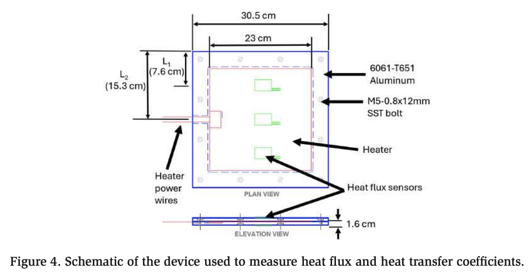
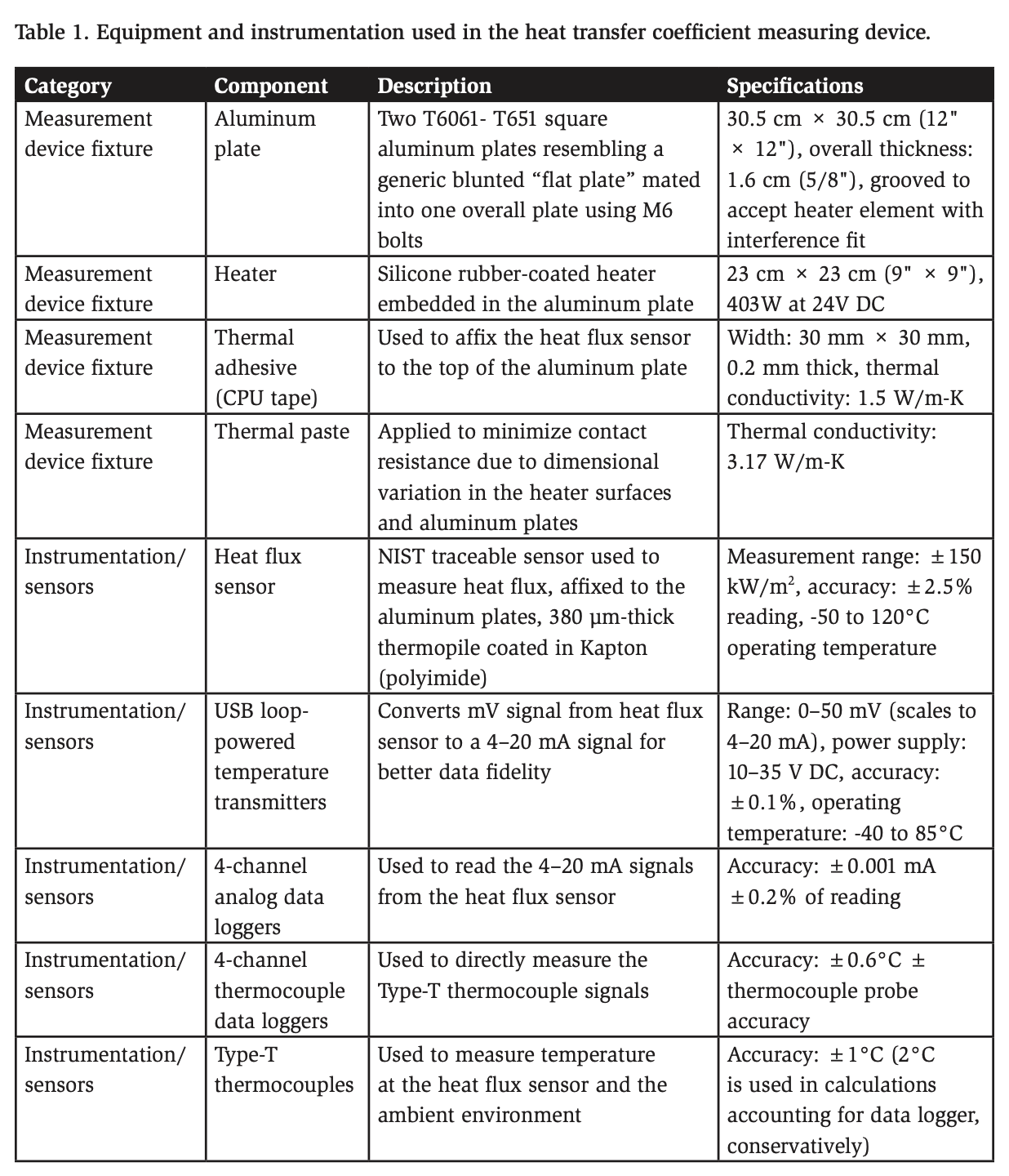
To measure the heat transfer coefficient in the five packaging plants considered in this study, an instrumented fixture was used to gather heat transfer data for the air flowing within a spiral freezer. The instrumented fixture comprised a pair of high-conductivity aluminum plates with dimensions similar to those of larger food products such as pizza. Figure 2 shows an illustration of the device, where a heat flux sensor is affixed to the top of the aluminum plates, is the heat flux measured through the heat flux sensor, is the estimated radiation, and T∞ is the temperature of the air in the environment.

The device configuration provided a durable surface for mounting heat flux and temperature sensors. The high thermal conductivity of aluminum, as opposed to the low conductivity of fruits, plaster, or plastic, minimized temperature gradients within the device, ensuring that the temperature measurements more accurately reflected the bulk temperature of the instrument. Heat flux sensors were secured using highconductivity thermal adhesive to minimize contact resistance between the sensor and the surface. An electric resistance heating element was embedded between the aluminum plates, allowing for the generation and maintenance of a controlled temperature difference between the surface and the surrounding airflow. This experimental device served as a pseudo-product and was sent on the same path that the products take in fully operational industrial spiral blast freezers at five different food processing plants.

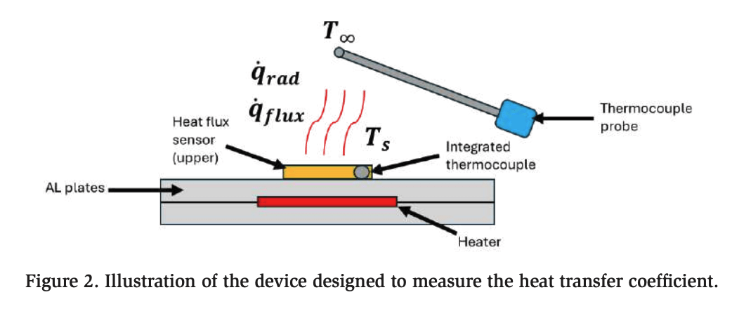
The illustration shown in Figure 2 includes a surface heat flux sensor, and Figure 3 shows a photo of the actual sensor used in the present work. This heat flux sensor was selected because it is NIST traceable and relatively inexpensive compared with other sensors that have a similar range and accuracy. The details of the chosen sensor and other instrumentation are provided in Table 1. The heat flux sensor outputs millivolt signals that vary based on the instantaneous heat flux through the sensor. The sensor was calibrated by the manufacturer using a guarded hot box apparatus and accompanied by a sensor-specific calibration curve of the millivolt output signal as a function of conduction heat transfer through the sensor. A Type-T thermocouple was integrated into the sensor, conveniently allowing the temperature that coincides with the heat flux sensor to be measured.

A single heat flux sensor was affixed to the top (leeward side) of the aluminum plate using double-sided thermal adhesive tape, commonly used for CPU applications. This adhesive was chosen for its durability, ease of use, and relatively high thermal conductivity compared with alternative mounting methods. The flat square geometry was used for the aluminum plate to simplify the design and calculations.

An embedded silicone heater was incorporated to maintain a temperature differential (ΔT) between the heat flux sensor and the ambient environment, enabling accurate heat flux measurements. A rectangular groove was machined into the interior of the aluminum plate to hold the silicone heater under slight compression, ensuring good thermal contact between the heater and the aluminum. Thermal paste was applied between the heater and the aluminum surfaces to reduce contact resistance caused by minor surface irregularities. Finally, the two halves of the aluminum assembly were securely bolted together, as illustrated in Figure 4.

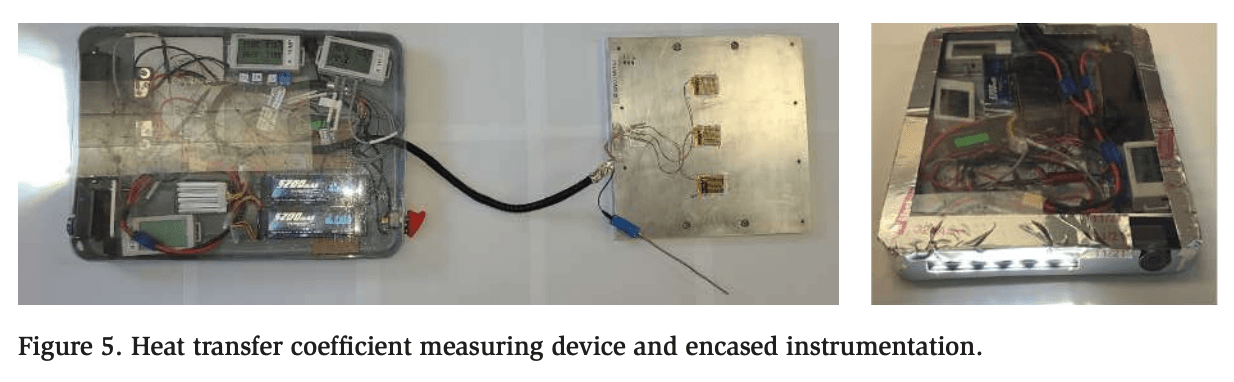
The millivolt signal generated by the heat flux sensor was converted to a 4–20 mA signal using loop-powered transmitters, following a simple scaling equation provided in the Appendix. The 4–20 mA signal demonstrated superior data fidelity when collected using the portable loggers compared with direct measurement and amplification of the millivolt signal. Additionally, compact battery-powered devices capable of measuring 4–20 mA signals are widely available, whereas devices with small millivolt signals are typically limited to thermocouple inputs. More versatile millivolt measurement devices are often bulky and require a power outlet. Portability was a key consideration, given the intended use of the instrument in a dynamic industrial air blast freezing system.

The signal transmitter used in this experiment is highly versatile and capable of operating with a wide power supply range from 10 to 35 V DC without compromising accuracy. This flexibility is particularly important because the transmitter is often powered by external batteries, which experience voltage drops over time owing to discharge in the harsh, low-temperature freezer environment. Type-T thermocouple signals were directly recorded using thermocouple data loggers. To ensure seamless data consolidation, all loggers were synchronized during initialization to the nearest second, aligning their timestamps for simple post-experiment analysis.

A durable action camera and LED lights were added to the measuring instrument to capture footage inside the spiral freezers and identify the precise location of the instrument at any given time. All of the components were packaged and fit inside a plastic enclosure, as shown in Figure 5.

As shown in Figure 2, a correction factor(ed b) was applied to remove radiation from the ( the measured flux, isolating the heat transfer caused by convection. The radiation correction resistance term (Rrad) was calculated using Equation 1, taken from Nellis & Klein (2009). The nomenclature of all the symbols and variables is listed in Table 3 in the Appendix.

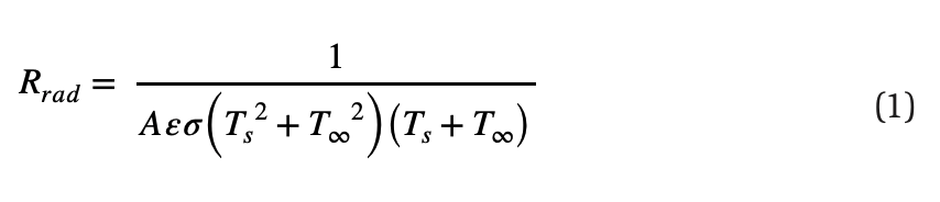
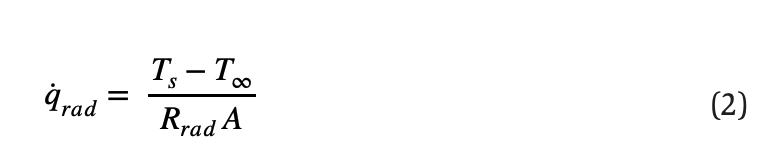
In Equation 1, A is the overall surface area of the plate, ε is the estimated emissivity of aluminum, and σ is the Stefan–Boltzmann constant (i.e., 5.67 × 10-8 W/m2 -K4 or 1.71 × 10-9 Btu/hr-ft2 -R4 ). A handheld infrared thermometer was used to measure the emissivity of the aluminum to be approximately 0.1, consistent with values typically observed for machined aluminum. Equation 2 shows the application of this radiation resistance in deriving a simple radiation correction factor qrad.

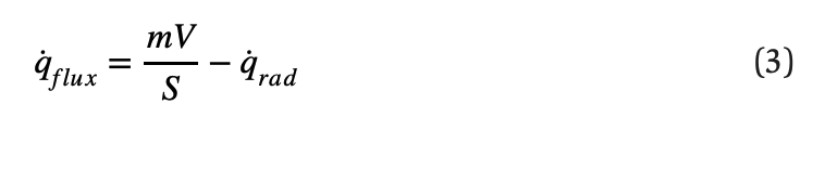
The heat flux for each sensor in W/m2 (or Btu/ft2 ) was then calculated using Equation 3, subtracting the radiation correction factor:

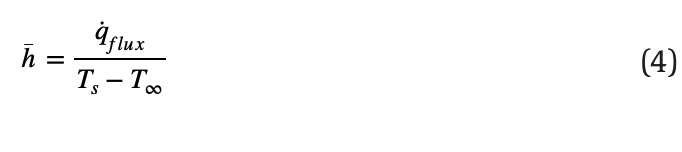
Finally, Newton’s law of cooling was used to calculate an effective local heat transfer coefficient:

Uncertainty calculations

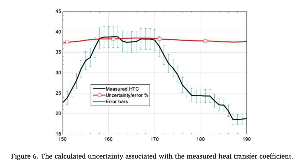
An uncertainty analysis was conducted to estimate the overall measurement accuracy of the surface heat transfer coefficient. Key components contributing to uncertainty included thermocouples, the heat flux sensor, and milliamp transmitters. The individual uncertainties for these elements were derived from manufacturer specifications or calibration data and were propagated through the calculations to determine their impact on the final heat transfer coefficient. As summarized in Table 2, the resulting uncertainty in the heat transfer coefficient was 14%.

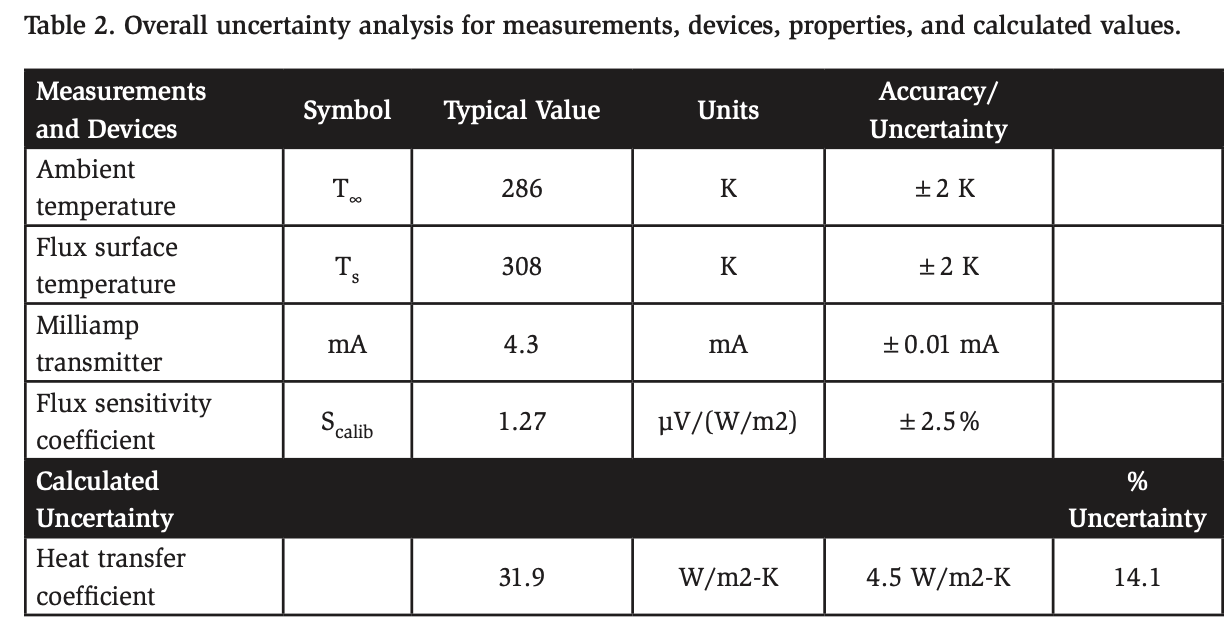
Figure 6 shows live data obtained in a spiral freezer, with the calculated uncertainty overlayed. In this example, the uncertainty is less than the listed value in Table 2 owing to the discrepancy in the temperature difference (ΔT) between the ambient spiral freezer air and the flux surface. The average error in the heat transfer coefficient is around 6.5% in Figure 6.

Results

Figure 7 presents the air temperature profiles of spiral blast freezers from five different plants, highlighting significant variability across locations. The data has been truncated at 1500 seconds to make comparisons between the different freezers easier. Plant 2 exhibits the coldest air, with an average temperature of approximately −38°F (−39°C), whereas Plant 1 exhibits the warmest air, averaging around −14°F (−26°C). Plants 3, 4, and 5 have similar air temperatures, approximately −25°F (−32°C). From a performance perspective, lower air temperatures are preferable because they enable faster freezing of the products. However, achieving lower temperatures necessitates lower saturated pressures within the refrigeration system, resulting in increased energy consumption. Therefore, optimal freezer performance requires a careful balance between air temperature and airflow to achieve the most efficient throughput.

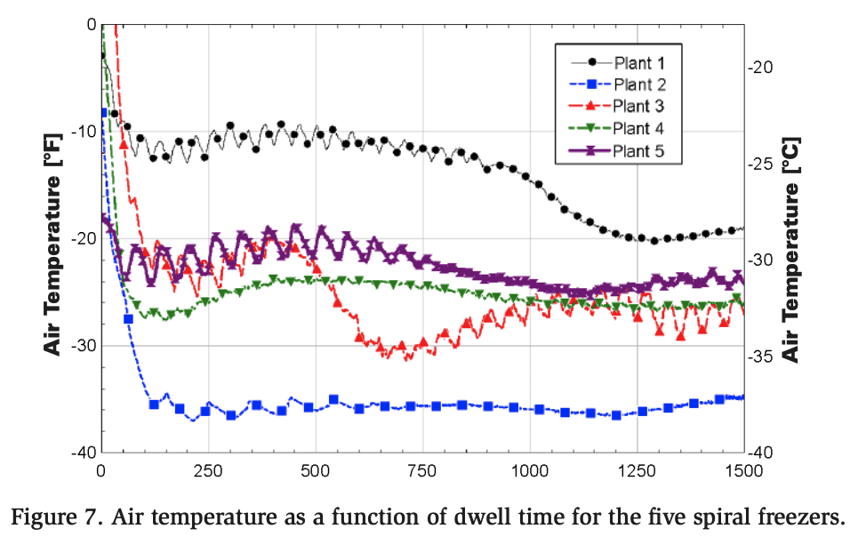
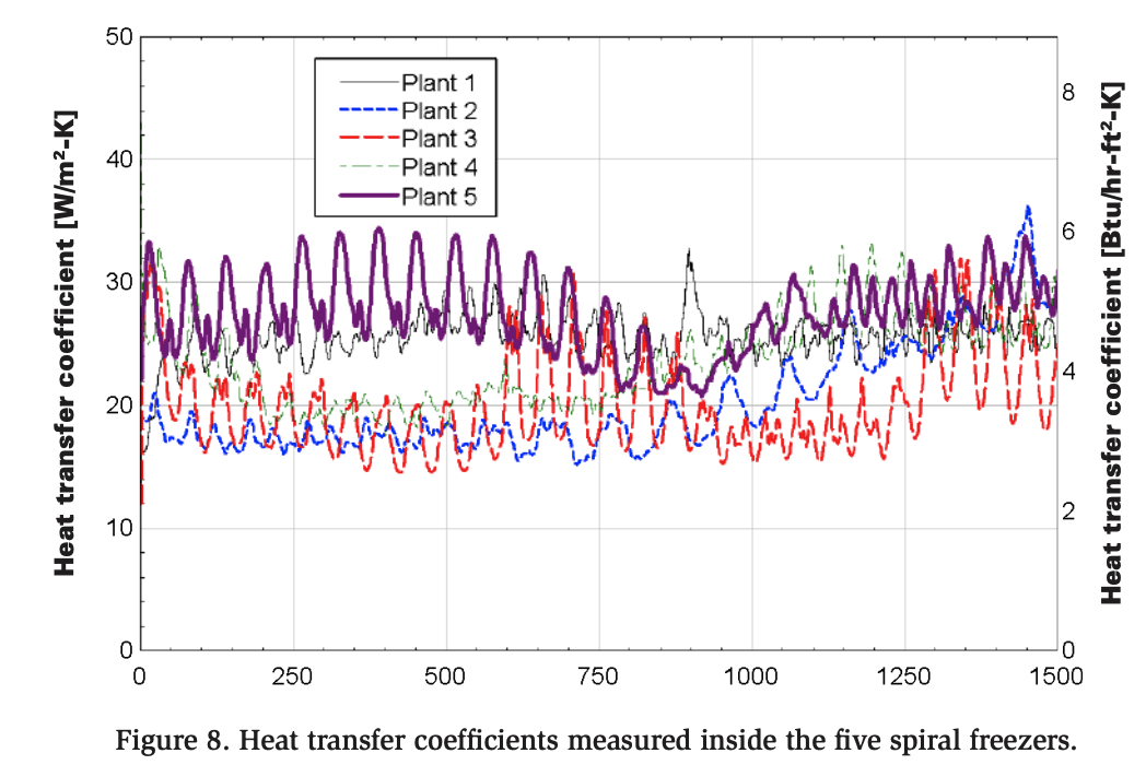
Figure 8 presents the measured heat transfer coefficients for all five spiral freezers, revealing distinct patterns across the plants. The data are presented utilizing an 8-point moving average to smooth out significant oscillations in the raw data, facilitating clearer visualization over the collection period. Plants 1 and 5 exhibit relatively high heat transfer coefficients at the start of the cooling process, which gradually taper to moderate values by the end. As discussed in a related paper, Optimizing Airflow in Spiral Blast Freezers (Alar, 2024), this is considered an optimal heat transfer profile for blast freezers. A higher heat transfer coefficient—indicative of greater air velocity—earlier in the cooling process enhances freezing efficiency.

In contrast, Plants 2, 3, and 4 begin with lower heat transfer coefficients. Plants 2 and 4 show some recovery by the end of the process, whereas Plant 3, which is considered to have the least desirable profile among the five facilities, maintains a consistently low value of around 20 W/m²-K (3.8 Btu/hr-ft²-°F). Despite Plant 2 having the coldest air temperature, it does not exhibit an ideal heat transfer profile, whereas Plant 5, with the most favorable velocity profile, only maintains moderate temperatures. An analysis is necessary to determine whether air temperature or airflow delivery plays a more critical role in the overall freezer performance.

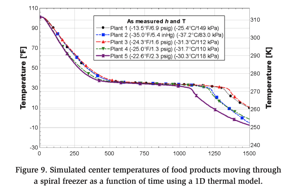
To evaluate the performance of each spiral blast freezer, the measured heat transfer coefficients and corresponding temperatures were applied as boundary conditions in a 1D thermal model of a food product moving through a spiral freezer. The results are presented in Figure 9, which also displays the saturation pressure of ammonia (R717) corresponding to the measured temperatures. The calculated center temperature of the food product upon exiting the freezer is included in the figure.

Among the freezers, Plant 5 demonstrated the best performance, achieving the most rapid cooling rate and an ideal heat transfer coefficient profile. Although Plant 2 exhibited a less favorable heat transfer coefficient profile, low air temperatures were obtained, performing nearly as well as Plant 5 by the end of the simulation (1500 seconds). In contrast, despite having a promising heat transfer coefficient profile, Plant 1 was one of the poorest performers, exhibiting higher air temperatures throughout the process.

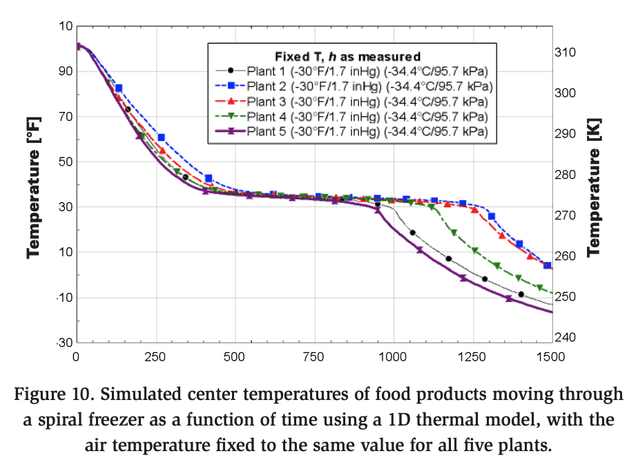
When the air temperatures are intentionally equalized across all five plants, the evaluation becomes solely dependent on the airflow velocity (heat transfer coefficient), as plotted in Figure 10. Notably, with the influence of air temperature removed, Plant 2 becomes the worst performer, but Plant 5 remains the top performer. Moreover, Plant 1 performs nearly as well as Plant 5 under these conditions, highlighting the significant impact of the velocity profile on freezer performance.

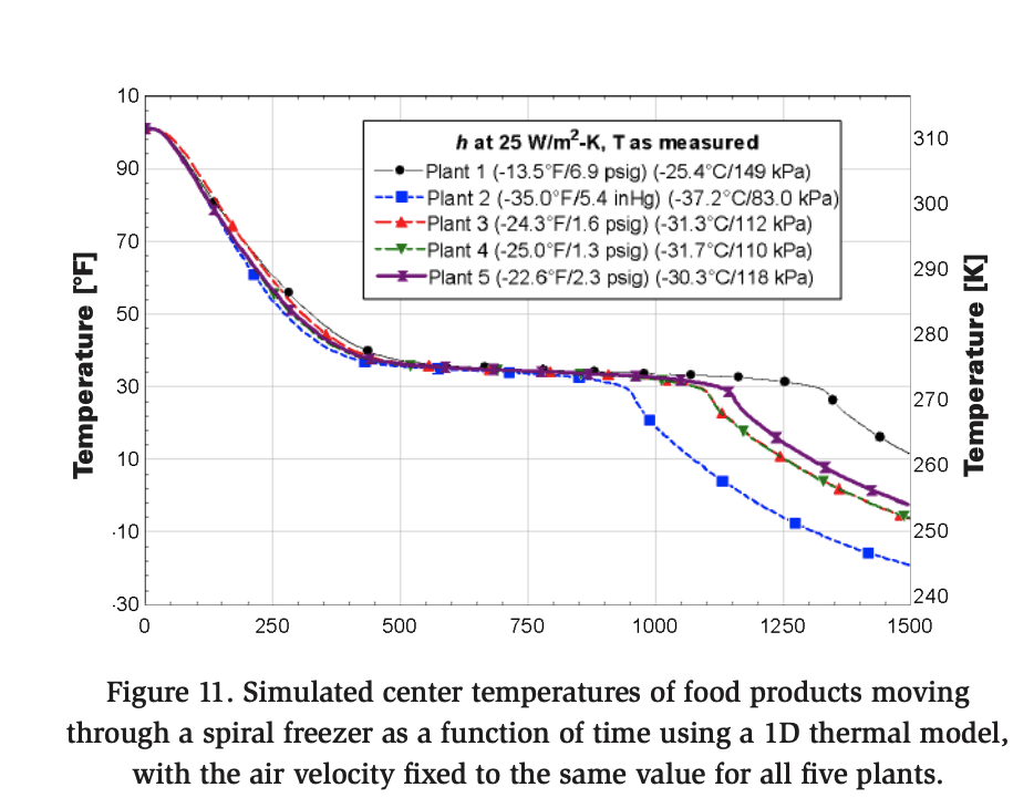
In the next analysis, the airflow velocity (heat transfer coefficient) is held constant across all five plants, allowing only the air temperature to vary based on the measured temperatures within each spiral freezer. The simulations are then repeated, as shown in Figure 11. The performance of the spiral freezers is directly correlated with air temperature, as illustrated in Figure 7. Plant 2, which had the lowest air temperature, achieved the lowest food center temperature, making it the top performer. In contrast, Plant 1, with the highest air temperature, was the poorest performer.

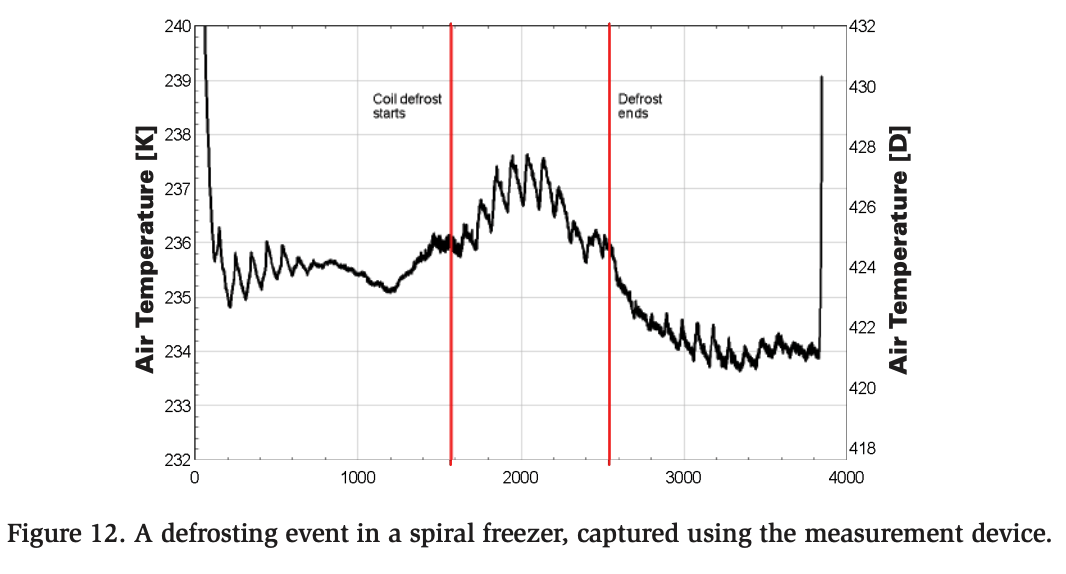
Additionally, the data obtained using the measurement device can be analyzed to examine the effects of defrosting and other phenomena on the air temperature inside a spiral freezer. Figure 12 shows the characteristics of a defrosting event captured using the measurement device.

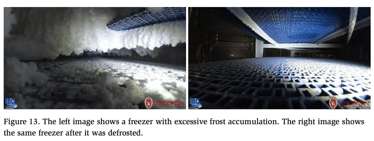
Finally, Figure 13 shows two images taken from a video captured using the action camera mounted on the measurement device. This visual feed serves as a valuable diagnostic tool for identifying operational anomalies such as excessive frost buildup, frost deposits, uneven belt transitions, and sanitation concerns. The left and right snapshots were taken at different points during the freezer’s operating cycle. The left image reveals significant frost accumulation, and the right image shows the same freezer after being warmed and defrosted a few days later, highlighting the difference in conditions before and after maintenance.

Conclusion

An instrumented fixture was developed for evaluating the thermal performance of dynamic air blast freezers by measuring heat transfer coefficients and air temperatures, as well as capturing diagnostic video in situ. The ability to gather realtime data while the device moves through the freezer alongside products enables the direct assessment and comparative analysis of freezer performance.

The airflow velocity (as indicated by the heat transfer coefficient) and air temperature can both be evaluated to determine freezer efficiency. Freezers with higher air velocities early in the cooling process, such as Plant 5, achieved greater performance despite having moderate air temperatures. Plant 2, with the coldest air temperature but suboptimal velocity profiles, performed moderately well, demonstrating that low temperature alone does not guarantee superior performance. These findings highlight the need to balance airflow velocity and air temperature for optimal energy and thermal efficiency.

In addition, video from the onboard action camera can provide valuable insights into operational anomalies, such as excessive frost buildup, uneven belt transitions, and sanitation issues. This visual feed, combined with thermal data, enhances the diagnostic capabilities of the system by identifying defrost events and operational irregularities in real time, as demonstrated in Figures 12 and 13.

Appendix

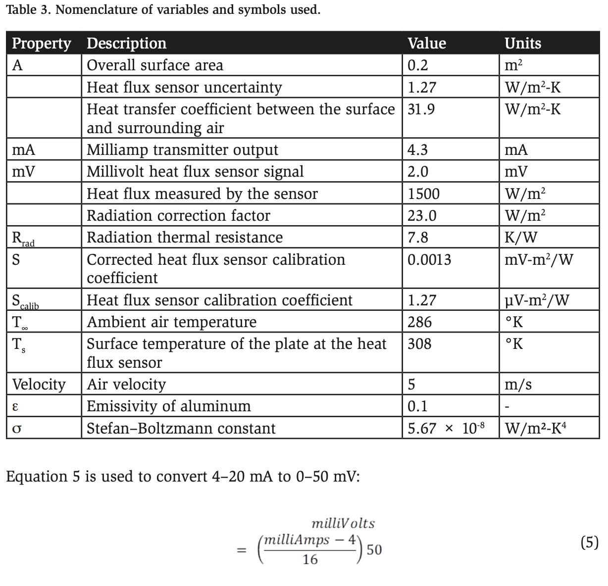
The calibration method used by the manufacturer of the heat flux sensor is based on an equation (Equation 6) that depends on the calibration sensitivity Scalib and surface temperature Ts . This sensitivity value varied from 0.00125 to 0.00134 mV/(W/m2 ) for all the flux sensors used herein. Equation 6 yields the overall sensitivity coefficient S:

References

Alar, E., Reindl, D., Nellis, G., & Young, T. (2024a). Optimizing airflow in Spiral Blast Freezers. International Journal of Refrigeration. https://doi.org/10.1016/j. ijrefrig.2024.07.015

Amarante, A., & Lanoisellé, J.-L. (2005). Heat transfer coefficients measurement in industrial freezing equipment by using heat flux sensors. Journal of Food Engineering, 66(3), 377–386. https://doi.org/10.1016/j.jfoodeng.2004.04.004

ASHRAE. (2018). 2014 ASHRAE Handbook: Refrigeration. Atlanta: American Society of Heating, Refrigerating and Air-Conditioning Engineers, Inc. ASHRAE. (2022). 2022

ASHRAE Handbook: Refrigeration. Atlanta: American Society of Heating, Refrigerating and Air-Conditioning Engineers, Inc.

Carson, James & Willix, Jim & North, Mike. (2006). Measurements of heat transfer coefficients within convection ovens. Journal of Food Engineering – J FOOD ENG. 72. 293-301. 10.1016/j.jfoodeng.2004.12.010. FluxTeq. (2024). PHFS-01 Heat Flux Sensor.

FluxTeq. Retrieved September 23, 2024, from https://www.fluxteq.com/phfs-01-heat-flux-sensor

HuksefluxUSA. (2024). FHF05 Foil Heat Flux Sensor. HuksefluxUSA. https:// huksefluxusa.com/products/thermal/fhf05/

Lemmon, E.W., and Jacobsen, R.T., “Viscosity and Thermal Conductivity Equations for Nitrogen, Oxygen, Argon, and Air”, International Journal of Thermophysics, Vol. 25, No. 1, January 2004, pp. 21-69

Lovatt, S.J., Pham, Q.T., Loeffen, M. and Cleland, A.C., 1993, A new method of predicting the time variability of product heat load during food cooling —part 2: experimental testing, J Food Eng, 18:13–36.

Omega. (2024). HFS-5 Thermocouple Type T Sensor (-50 to 120°C). Newark. https:// www.newark.com/omega/hfs-5/thermocouple-type-t-50-to-120deg/dp/32AK5426

Nellis, G., & Klein, S. A. (2009). Heat transfer. Cambridge University Press.

Mannapperuma, J. D., Singh, R. P., & Reid, D. (1994). Effective surface heat transfer coefficients encountered in air blast freezing of whole chicken and chicken parts, individually and in packages. International Journal of Refrigeration, 17(4), 263–272. https://doi.org/10.1016/0140-7007(94)90043-4

Reynoso, R., & Calvelo, A. (1985). Comparison between fixed and fluidized bed continuous pea freezers. Revue Internationale Du Froid, 8(2), 109–115. https://doi. org/10.1016/0140-7007(85)90083-0

FAO “Energy-Smart Food for People and Climate, United Nations, Food and Agriculture Organization (FAO), (2011).