


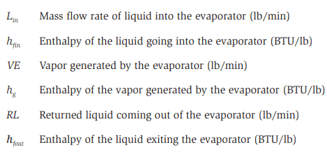
Simple Equations for Determining Mass Flow in Refrigeration Systems
DON FAUST, TRAINING MANAGER, FRICK, A JOHNSON CONTROLS COMPANY
ABSTRACT
The goal of any industrial refrigeration system is to remove heat. Therefore, the total heat load is the design engineer’s first calculation, which is then used to size and select the evaporators. Unfortunately, this heat load is often also applied to the sizing of other components in the system, which can result in errors. However, heat load should only be used to size components that exchange heat. This paper introduces a methodology and develops simple equations for determining mass flows in industrial refrigeration systems. The proposed methodology involves the mass balance technique, which assumes a steady-state condition in which the sum of the mass flows into a machine or system equals the sum of the mass flows out. The mass balance technique can help quantify mass flows that may be difficult to calculate using other methods. The mass flow equations apply to any refrigerant in a typical vapor compression cycle. Modern industrial refrigeration systems often employ multiple temperature and pressure levels to maintain various conditions in processing and storage facilities. Mass balances enable the accurate sizing of various pieces of equipment, and this technique can reveal strategies for saving energy and initial cost.
Introduction
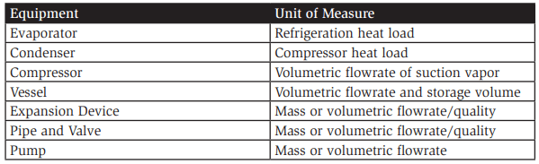
When designing an industrial refrigeration system, the first calculation determines how much heat must be removed and at what temperature. The evaporator load is the first “hard number” a system designer calculates, and the rest of the system follows from there. The ton of refrigeration (TR) unit is used to describe a heat transfer rate, particularly applicable to evaporators. Sizing all the equipment in an industrial refrigeration system based on the evaporator heat load (i.e., one number does it all) would be convenient. Often, designers do precisely that: select non-heat exchanging equipment using a rate of heat exchange. The sizing tables published by manufacturers imply that evaporator load is a valid method for sizing all industrial refrigeration equipment. Virtually every component in a refrigeration system has a table or chart showing its “capacity” in TR (or kW). Pipes, vessels, pumps, compressors, and valves have manufacturer- and industrypublished capacities in units of heat transfer. These tables include footnotes, typically in small print, listing the assumptions, which should prevent the designer from using the wrong units of measure to size their equipment. By examining the equipment in an industrial refrigeration system, the units for sizing the equipment are clearly essential to the equipment’s function. For example, a compressor can be viewed as a gas volume reduction device, revealing the fundamental unit for compressors—volumetric flow rate. Vessels for separation can be considered fat spots in the pipe where the vapor is slowed down. Thus, volumetric flow is a proper determiner for vessel size. Note that vessels may also require a holding capacity independent of liquid–vapor separation requirements.
Proper Units for Selecting Equipment
In an industrial refrigeration system, the proper units for most of the equipment are not related to the heat transfer occurring in the evaporators. A mass balance reveals the mass flows for every piece of equipment in the system, which can be converted into the proper units of measure to size each component.
Mass Balance Equation
![]()
The problem-solving technique of mass balance centers around the concept that mass flow in equals mass flow out at steady-state conditions for a system or sub-system. In a chemical process, numerous factors can change the physical state of the refrigerant, which significantly affects the volume, but the mass flows must still balance. Every part of the system has a mass flow of refrigerant in and out, and the sum of the flows into and out of each piece of equipment must be equal. Mass balance applies to any single piece or group of pieces of equipment. Mass in must equal mass out under steady-state conditions.
Are Refrigeration Systems Steady-state?
Many examples of non–steady-state circumstances are related to refrigeration systems, including spiral freezers starting up in the morning, condensers that fill with liquid, and receivers that run dry. Do these empirical observations disprove the steady-state assumption for refrigeration systems? The answer is both yes and no. Yes, the steady-state assumption does not account for system upsets, making it invalid for brief periods. However, the longer the duration, the more valid the steady-state assumption. A mass imbalance can only be present for a short period for the steadystate assumption to apply, which is the case in industrial refrigeration systems. Flash Gas Problem One issue with using evaporator load to size other equipment is accounting for the non-useful work of flash gas (FG). This is not an issue with single-temperature systems, as flash gas is typically considered in the manufacturers’ catalog ratings. When the system has multiple suction temperatures and each level removes FGs for the lower temperature levels, the system cannot be accurately sized using evaporator load.
Most industrial refrigeration systems have multiple suction temperatures, and how they handle FG is based on system efficiency. Performing a system mass flow balance is an effective way to account for FG in a multiple-temperature system properly.
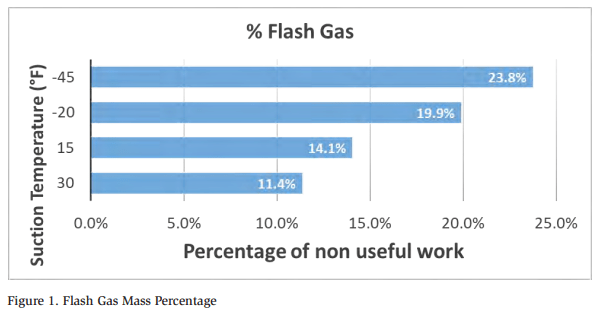
FG is not an insignificant load. Figure 1 shows that FG accounts for 1/8 to 1/4 of the total mass flow to the compressors of a refrigeration system, depending on the suction temperature, highlighting the need for mass balances. FG is the next major load after the refrigeration load itself, and it is too significant to be subjected to guesses. When multi-temperature systems are used, a mass balance can accurately calculate how much FG occurs at each temperature level.
The condensing temperature used in these calculations is 85°F. While 95°F is commonly used to size condensers, it is based on 0.4% of one day. Most systems run at around 85°F, condensing most of the time, so this temperature is sufficient for analyzing typical, not worst-case, operation.
Thermodynamic Calculations
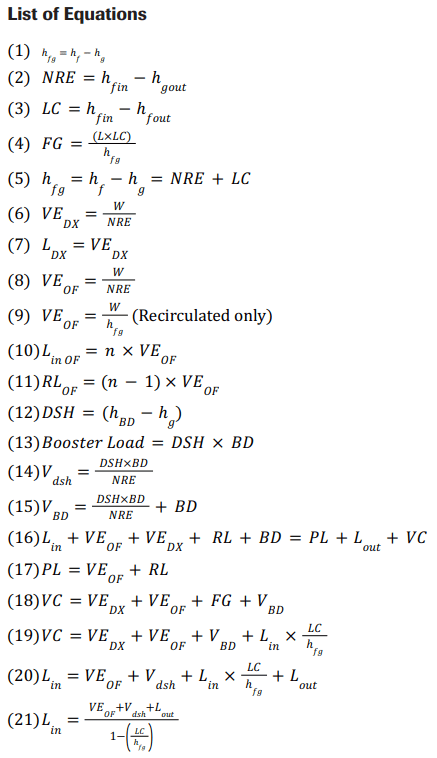
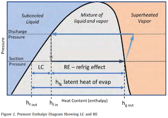
Latent heat of evaporation, FG, and net refrigerating effect (NRE) are terms that are familiar to the refrigeration engineer. Liquid cooling (LC) is a term used to quantify the FG “load.” Figure 2 depicts the LC, RE, and latent heat terms. Note that all thermodynamic equations are listed in the appendix.
Latent Heat of Evaporation
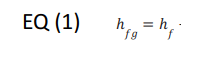
The latent heat of evaporation hfg is the difference in enthalpy between saturated liquid and saturated vapor at a constant temperature. This value, often listed in thermodynamic tables, can be calculated by subtracting the enthalpy of the saturated liquid hf from the enthalpy of the saturated vapor hg at the temperature and pressure under consideration:
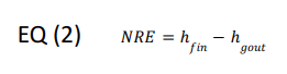
Net Refrigerating Effect
The NRE is the difference in enthalpy between the entering liquid hfin and the saturated vapor hgout in the process under consideration, as shown in EQ (2). The absolute value of this term is commonly used.
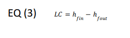
Liquid Cooling
Work, in the form of mechanical cooling, occurs when the temperature of a liquid refrigerant decreases within a closed system. For example, warm liquid entering a cold evaporator must be cooled to its saturation temperature. This cooling load, called LC, is the difference between the entering liquid’s enthalpy hfin and the leaving liquid’s enthalpy hfout:
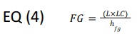
Flash Gas
FG is the vapor generated when cooling the incoming liquid to the saturated temperature in the process being examined. The FG calculation requires NRE and LC. The FG load is the product of the mass flow rate of the liquid L and the LC enthalpy difference. The FG mass flow is simply equal to that load divided by the latent heat of evaporation:
Breaking Down Latent Heat of Evaporation
Evaporation always occurs at saturation. However, not all processes in a refrigeration system occur with saturated liquid and saturated vapor. For example, if warm liquid enters a cold evaporator, the liquid must cool to saturation before it can evaporate, known as LC. The net thermodynamic result of cooling the liquid to saturation with subsequent evaporation is called the NRE. The latent heat of evaporation is considered as the sum of the NRE and the LC:
![]()
Mass Flow for Evaporators
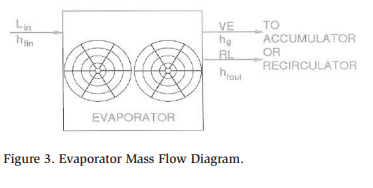
Evaporator mass flows vary depending on the type of evaporator feed being used. Two assumptions are made: all evaporators take in liquid, and what exits is either a vapor or a mixture of vapor and liquid. Figure 3 shows an evaporator mass flow diagram.
Two scenarios are examined:
DX Feed
Liquid enters the evaporator through a direct expansion (DX) device, and it is flashed down to the evaporating temperature. The vapor exiting the evaporator is dry. All the liquid fed to the evaporator evaporates, leaving no returned liquid (RL) (i.e., RL = 0).
Overfed (Pumped or Flooded) Feed
The liquid is flashed down to the evaporator temperature in the recirculator, then pumped to the unit. The liquid enters at the evaporation temperature; therefore, no FG is generated at the evaporator. The vapor exiting the evaporator carries the overfed liquid.
DX Feed Evaporators
No RL is present because the suction coming out of a DX evaporator is dry. For calculation purposes, the expansion device is considered to be a part of the evaporator. For DX, the recirculation ratio n is one.
The vapor generated by the evaporator is the refrigeration load divided by the NRE.
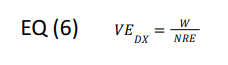
where W is the refrigeration load (BTU/min). To convert TR to BTU/min, multiply by 200.
Most DX systems utilize superheat in the vapor to control the amount of liquid feed. This superheat performs useful work in cooling. To properly account for the superheat’s contribution, use hg for the superheated condition in the NRE calculation. However, if the superheated vapors meet saturated liquid later in the system, such as in a wet return pipe or a vessel, the superheated vapors are cooled to saturation. In this case, the net effect to the system would be the same, using the enthalpy for saturated gas at evaporation. The examples for mass balance use this approximation—saturated conditions are used at the outlet of the DX evaporator.
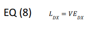
The liquid supplied to the evaporator is
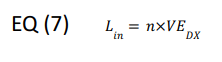
For DX evaporators, n = 1. Therefore, EQ (7) becomes
Note that DX evaporators typically receive their liquid from one vessel and return the vapor to another. For example, the high-pressure receiver feeds the liquid to the evaporator, and the vapor flows to the accumulator. This information is critical when doing vessel mass balances. Most DX evaporators feed from the high-pressure receiver, but some may feed from a different source, and their liquid feed must be added to the liquid flowrate out Lout for the vessel supplying the liquid.
Overfed Evaporators (Pumped or Flooded)
Overfed evaporators feed more liquid than they evaporate. Often, this liquid is fed to the evaporator as a saturated liquid—the FG is taken off in the recirculator vessel, and the liquid is pumped to the evaporator. In these cases, the evaporator can use the entire latent heat of evaporation rather than just the NRE. The downside to this approach is that the return piping must carry both the vapor generated by the evaporator and the overfed liquid.
Circulation Ratio
The industrial refrigeration industry uses many terms for circulation ratio, including overfeed rate, overfeed ratio, recirculation ratio, circulating number, and circulating rate. However, the definition of the concept remains the same in textbooks and handbooks, as illustrated in Figure 4.
Page 302 of Will Stoecker’s “Industrial Refrigeration Handbook” defines the circulation ratio n as
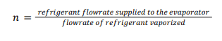
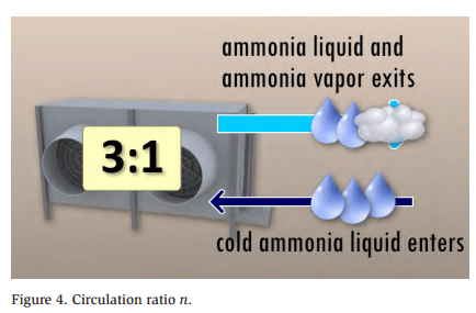
The ASHRAE Refrigeration Handbook, 1990, page 2.3, states: “In a liquid overfeed system; the mass ratio of liquid pumped to the amount of vaporized liquid is the circulating number or rate.” The circulation ratio defines the quality of the refrigerant at the outlet of the evaporator. A vapor quality of 50% implies a 2:1 circulation ratio. Likewise, if the vapor quality is 33%, the circulation ratio is 3:1. This simple ratio of the amount of vapor generated to the amount of liquid fed to the evaporator is the inverse of the vapor quality.
One difference between CPR and pumped systems is the temperature of the liquid fed to the evaporators. In a pumped system, the liquid is at its saturation temperature in the recirculator, where the pump pressurizes it (in effect making it a subcooled liquid) and pushes the saturated liquid out to the evaporators.
The vapor generated by the evaporator (see Figure 3) is calculated as
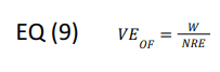
Equation (9) applies to flooded or recirculated feeds. However, for a pumped recirculated feed, the NRE is the same as hfg. Thus, for recirculated loads, EQ (9) can be simplified to
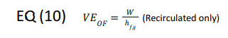
For cases in which the pumped or pressure-fed liquid is not at saturated conditions for the evaporator (i.e., in CPR systems), using the NRE (EQ (9)) is more appropriate, even though NRE = hfg for many applications.
The liquid supplied to the evaporator is calculated as
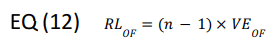
Additionally, the returned (overfed) liquid (RL) is calculated as
Vessel Mass Flow
Mass balances can be applied to any component in the industrial refrigeration system. However, the vessels are the critical components when solving the mass flows for the system. The vessels are central in terms of flow—they receive the mass flows from the evaporators, they often produce FG, and the compressors pull vapor from the vessels. The vessels in the system require an understanding of where FG is removed so that the compressors can be sized properly.
The mass flow VE of vapor generated by the evaporators is required before achieving a system mass balance. This mass flow, which performs useful work, accounts for 80% of the vapor generated by the system. The remaining 20% of vapor is FG, which does not do useful work.
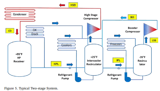
The most efficient way to organize a system is to have the liquid from the condensers flow through each temperature in the system successively. Higher-temperature vessels feed the liquid to the next lower-temperature vessel. That way, the liquid is flashed off in steps until it gets to the lowest temperature in the system. Note that the liquid fed to the −35°F vessel comes from the +25°F intercooler. The liquid from the HP receiver is first cooled to +25°F, then to −35°F.
The system shown in Figure 5 is a two-stage intercooled system. This generalized method applies to any refrigerant and both single-and two-stage systems. In a single-stage system, the booster discharge (BD) mass flows are zero. For a two-stage intercooled system, the system may look like Figure 5.
Vessel Mass Flow Equations
For any piece of equipment, the following must be true:
![]()
The methodology described herein applies to any vessel (except for a CPR with cold liquid return). This generalized approach includes a provision for an intercooler; if the vessel does not do intercooling, the corresponding parameters are zero.
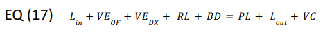
The sum of all the flows in minus those out equals zero. The mass flows are listed below and illustrated in Figure 6:
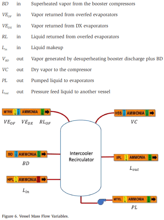
The vapor mass flow VE generated in the evaporators and the liquid makeup Lin to the vessel are independent of the overfeed rate. The overfeed rate is introduced to the calculations for pumping rate PL and the amount of liquid returned RL in the wet suction header. The vapor flow to the compressor VC is simply the sum of VE, the cooling performed on the discharge gases Vdsh, BD, and any flash loads.
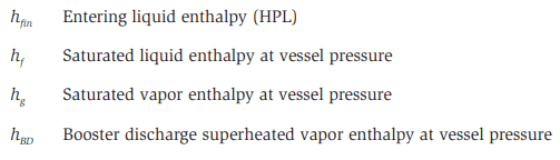
Thermodynamically, four enthalpies are of concern:
The first step in solving for mass flow is to use EQ (2) and EQ (3) to determine NRE and LC.
Intercoolers
If the vessel under consideration is an intercooler, then EQs (13)–(16) apply. If the vessel is not an intercooler, these values are zero.
For an intercooler, the high-stage compressors must recompress the low-stage mass flow and take in the vapor generated by desuperheating the BD gases. For this example, the BD gas is assumed to be desuperheated to saturated conditions by using the saturated enthalpy hg. If this is not the case, use the expected enthalpy at the gas condition.
Booster Gas Load to High Stage
The booster gas load considers the enthalpy difference between the superheated BD gas and the saturated gas:
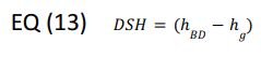
Multiply the result of EQ(13) by the mass flow to obtain the load:
![]()
where BD is the mass flow from the low-stage compressors (lb/min or kg/min). Vapor generated by desuperheating is the booster load divided by the NRE.
![]()
For the intercooler, the NRE is the enthalpy difference between the saturated vapor in the intercooler and the makeup liquid (typically HPL). The mass flow from the BD is then added to the desuperheating load for the total BD load.
![]()
Vessel Overall Mass Balance
The first intercooler equation is a mass balance. The masses entering the vessel are Lin, VE, RL, and BD. The masses leaving the vessel are the pumped liquid PL, Lout, and VC. The sums of mass into and out of an intercooler should be equal.
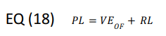
Pumped Liquid
The mass flow of pumped liquid PL going out, in terms of mass flow, equals the mass flow of VE plus that of the RL:
Vapor to the Compressor
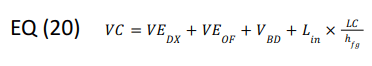
The load to the compressors is the sum of VE, the FG mass flow from the incoming liquid, and the BD load. Vapor to the Compressor
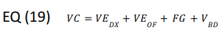
Using EQ (4), for FG, EQ (19) can be rewritten:
Makeup Liquid
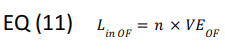
The amount of makeup liquid is equal to the amount of vapor evaporated by the overfed evaporators, the desuperheating vapor to the intercooler, the FG generated by the makeup liquid, and any liquid fed downstream (Lout).
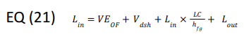
No DX loads need to be considered, so only the evaporated portion of the evaporator load is included in the liquid feed.
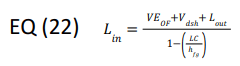
Since Lin exists on both sides of EQ (21), solving EQ (21) for Lin produces EQ (22):
Pressure Feed to Downstream Vessels
Solving for liquid out Lout is not possible. The value of Lout must be known before solving the rest of the equations. Thus, the solution begins at a vessel in which Lout is known—at the lowest-temperature vessel in the system, where Lout is zero.
In other words, all analyses must start with the lowest-temperature vessel in the system and move up from there. The mass flow Lin for the lowest-temperature vessel equals Lout for the next lowest-temperature vessel, and so on.
This model assumes that DX liquid comes from the high-pressure receiver. If the DX feed liquid comes from another source (i.e., a different vessel), then simply add that amount of liquid to the Lout for that vessel.
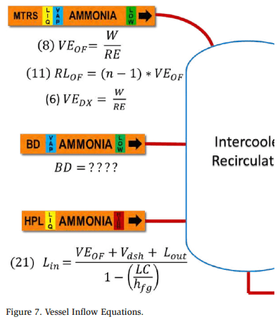
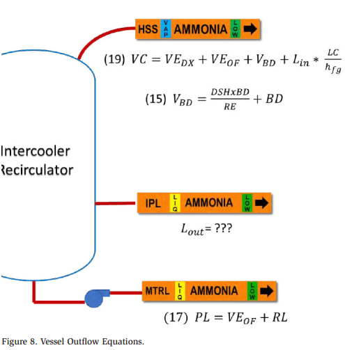
Vessel Inflows and Outflows
Figures 7 and 8 illustrate the vessel inflow and outflow equations
Applying Mass Balances to Systems
To perform the mass balance, the following information is needed:
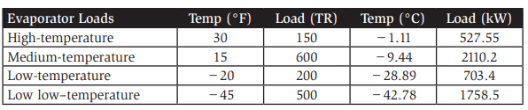
- Evaporator loads
- Respective system temperatures and pressures
- Style of feed for the sets of evaporators
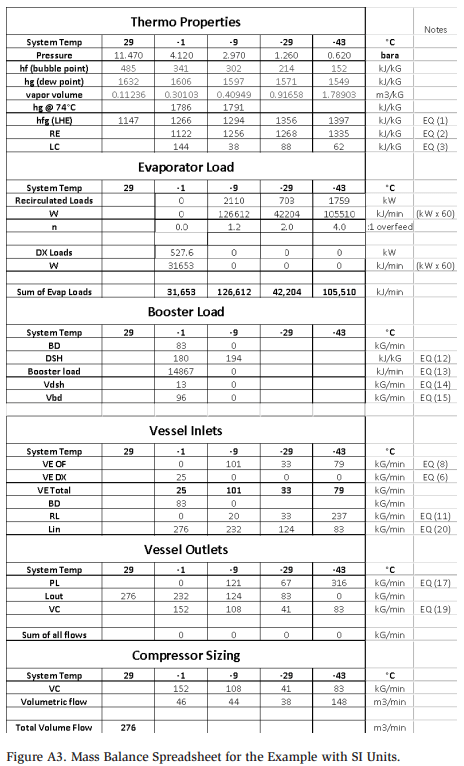
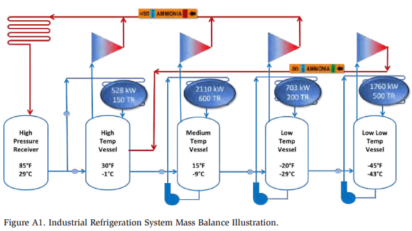
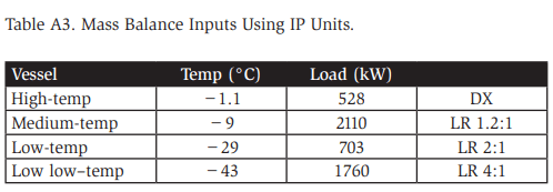
Then, using the thermodynamic properties of the refrigerant, the rest of the calculations can be performed. A multiple-temperature system consisting of four temperature levels, including a twostage component for the low low–temperature load, will be analyzed. The evaporator loads are as follows:
The appendix shows the results of a spreadsheet analysis of the system using both imperial (IP) and SI units. Note that the analysis must begin with the lowesttemperature vessel in the system and move up from there.
Conclusion
Mass balances are simple to perform, requiring only an hour or two of spreadsheet programming, and these equations can be used to solve for any refrigerant at any temperature. Unfortunately, although easy to do, many systems are designed without mass balances. However, if the user carefully reads the fine print on the ratings, a system can be designed using evaporator loads only with near-accurate results. For many industrial refrigeration systems, near-accuracy is not sufficient, especially when a mass balance can be performed to obtain more realistic loads in the system. With computers and spreadsheets available, every system should have a mass balance.
Appendix
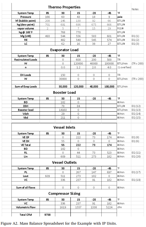
Mass Balance Example—IP Units
The mass balance example for this system consists of four refrigeration levels. The receiver is assumed to be at normal operating conditions (85°F condensing). The loads are shown in Table A1:
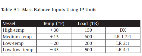
Note that the low low–temperature system is two-stage, and it discharges into the high-temperature vessel.
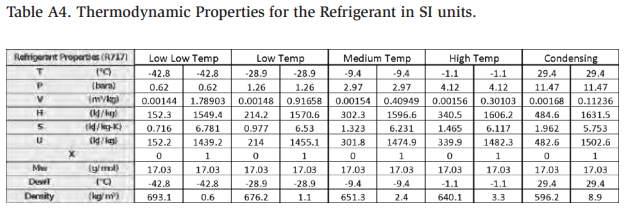
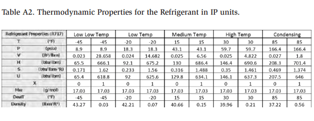
The thermodynamic properties of the refrigerant at the selected design temperatures (courtesy of FRICK CoolWare) are shown in Table A2. Figure A2 shows a snapshot of the spreadsheet program solving the mass balance with IP units.
Mass Balance Example—SI Units
This mass balance example is for the same system consisting of four refrigeration levels. The receiver is assumed to be at normal operating conditions (29°C°F condensing). The loads are shown in Table A2:
The thermodynamic properties of the refrigerant at the selected design temperatures (courtesy of FRICK CoolWare) are shown in Table A4: